Reports
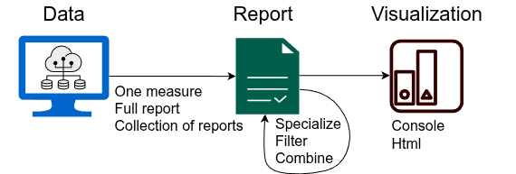
Reports perform multi-faceted analyses of AI system outcomes (e.g., predictions, recommendations, regression scores) that typically quantify biases and fairness. Intermediate computations are retained so that you can specialize to viewing sub-reports or computation internals. Furthermore, filters can be applied to augment the organization or apply rules (e.g., thresholding criteria) to report outcomes. The end-result is shown using various visualization environments.
To sum up, reports are structures that you can iterate on and explore. This way, you can move from summary values to computational details. Everything computed by FairBench is a report, be it one measure value, the report types described in this document, or even collections of reports for comparing datasets and algorithms across variations and time.
Tip
A more to-the-point tutorial than this documentation can be found in the full report overview. Here we we focus on filling details of the programmatic interface.
Report types
Out-of-the box, use one of the following report generation methods:
| Report | Description |
|---|---|
fb.pairwise |
Compares groups pairwise when needed. |
fb.vsall |
Adds the whole population as an 'all' group and, when possible, defaults to measures that compare other groups to 'all'. |
fb.conflate |
Creates a conflation matrix (a generalization of the confusion matrix whose entries are pairwise reports) between each subgroup pair. Values of these comparisons are not aggregated but instead retained as they are. |
Glimpse below example usage if the first report type for a binary classification task. Report types are interoperable; the other two can be called by just substituting their name in the same workflow. Of course, with different results.
Arguments, specialization,
and visualization are discussed afterwards in this document.
The example task contains binary predictions, binary
ideal predictions and multiclass
sensitive dimensions sensitive that separate between
men and women. The show method is used
to print the report to the console in a simple yet verbose
format. This is the default visualization environment.
Other visualizations
look very different and can be customized.
import fairbench as fb

sensitive = fb.Dimensions(men=[1, 1, 0, 0, 0], women=[0, 0, 1, 1, 1])
report = fb.reports.pairwise(
    predictions=[1, 0, 1, 0, 0],
    labels=[1, 0, 0, 1, 0],
    sensitive=sensitive
)
report.show()
##### multidim ##### |This is analysis that compares several groups. | |Computations cover several cases. ***** min ***** |This reduction is the minimum. |Computations cover several cases. (0.0, 0.5) ▎ █ ▎ █ █ █ █ ▎ █ █ █ █ ▎ * - + x o □ ◇ # @ % & | ▎ ▎▬▬▬▬▬▬▬▬▬▬▬▬▬▬▬▬▬▬▬▬▬▬▬▬▬▬▬▬▬▬▬▆▬▬▆ (12.0, -0.5000000000000001) * acc 0.333 min acc - pr 0.333 min pr + tpr 0 min tpr x tnr 0.500 min tnr o ppv 0 min ppv □ f1 0 min f1 ◇ gmi 0 min gmi # tar 0 min tar @ trr 0.333 min trr % lift 0 min lift & mcc -0.500 min mcc | kappa -0.500 min kappa ***** max ***** |This reduction is the maximum. |Computations cover several cases. (0.0, 2.0) ▎ █ ▎ █ ▎ █ ▎ █ ▎ ▄ ▄ ▄ █ ▎▬*▬▬-▬▬+▬▬x (4.0, 0.0) * pr 0.500 max pr - tar 0.500 max tar + trr 0.500 max trr x lift 2 max lift ***** maxerror ***** |This reduction is the maximum deviation from the ideal value. |Computations cover several cases. (0.0, 1.5) ▎ █ █ ▎ █ █ ▎ █ █ █ █ █ █ ▎ ▄ █ █ █ █ █ █ ▎ █ █ █ █ █ █ █ █ ▎▬*▬▬-▬▬+▬▬x▬▬o▬▬□▬▬◇▬▬# (8.0, 0.0) * acc 0.667 maxerror acc - tpr 1 maxerror tpr + tnr 0.500 maxerror tnr x ppv 1 maxerror ppv o f1 1 maxerror f1 □ gmi 1 maxerror gmi ◇ mcc 1 maxerror mcc # kappa 1 maxerror kappa ***** wmean ***** |This reduction is the weighted average. |Computations cover several cases. (0.0, 0.8) ▎ █ ▎ █ █ ▎ ▄ █ █ ▎ █ █ █ █ █ █ █ ▎ █ █ █ █ █ ▄ █ █ ▎▬*▬▬-▬▬+▬▬x▬▬o▬▬□▬▬◇▬▬#▬▬@ (9.0, 0.0) * acc 0.600 wmean acc - pr 0.400 wmean pr + tpr 0.400 wmean tpr x tnr 0.700 wmean tnr o ppv 0.400 wmean ppv □ tar 0.200 wmean tar ◇ trr 0.400 wmean trr # lift 0.800 wmean lift @ kappa 0.100 wmean kappa ***** mean ***** |This reduction is the average. |Computations cover several cases. (0.0, 1.0) ▎ █ ▎ █ ▎ █ ▄ █ ▎ █ ▄ █ █ █ █ █ ▄ █ ▎ █ █ █ █ █ █ █ ▄ █ █ ▄ ▂ ▎▬*▬▬-▬▬+▬▬x▬▬o▬▬□▬▬◇▬▬#▬▬@▬▬%▬▬&▬▬| (12.0, 0.0) * acc 0.667 mean acc - pr 0.417 mean pr + tpr 0.500 mean tpr x tnr 0.750 mean tnr o ppv 0.500 mean ppv □ f1 0.500 mean f1 ◇ gmi 0.500 mean gmi # tar 0.250 mean tar @ trr 0.417 mean trr % lift 1 mean lift & mcc 0.250 mean mcc | kappa 0.250 mean kappa ***** gm ***** |This reduction is the geometric mean. |Computations cover several cases. (0.0, 0.7071067811865476) ▎ █ ▎ ▆ █ ▎ █ █ ▎ █ ▂ █ ▂ ▎ █ █ █ █ ▎▬*▬▬-▬▬+▬▬x▬▬o▬▬□▬▬◇▬▬#▬▬@▬▬% (10.0, 0.0) * acc 0.577 gm acc - pr 0.408 gm pr + tpr 0 gm tpr x tnr 0.707 gm tnr o ppv 0 gm ppv □ f1 0 gm f1 ◇ gmi 0 gm gmi # tar 0 gm tar @ trr 0.408 gm trr % lift 0 gm lift ***** pnorm ***** |This reduction is the p-norm (default L2). |Computations cover several cases. (0.0, 2.0) ▎ █ ▎ █ ▎ █ ▎ █ █ ▂ █ █ █ █ ▂ ▂ ▎ █ ▆ █ █ █ █ █ ▄ ▆ █ █ █ ▎▬*▬▬-▬▬+▬▬x▬▬o▬▬□▬▬◇▬▬#▬▬@▬▬%▬▬&▬▬| (12.0, 0.0) * acc 1 pnorm acc - pr 0.601 pnorm pr + tpr 1 pnorm tpr x tnr 1 pnorm tnr o ppv 1 pnorm ppv □ f1 1 pnorm f1 ◇ gmi 1 pnorm gmi # tar 0.500 pnorm tar @ trr 0.601 pnorm trr % lift 2 pnorm lift & mcc 1 pnorm mcc | kappa 1 pnorm kappa ***** maxrel ***** |This reduction is the maximum relative difference. |Computations cover several cases. (0.0, 1.0) ▎ █ █ █ █ █ █ ▎ █ █ █ █ █ █ ▎ █ █ █ █ █ █ █ ▎ █ █ █ █ █ █ █ █ █ ▆ ▎ █ █ █ █ █ █ █ █ █ █ █ █ ▎▬*▬▬-▬▬+▬▬x▬▬o▬▬□▬▬◇▬▬#▬▬@▬▬%▬▬&▬▬| (12.0, 0.0) * acc 0.667 maxrel acc - pr 0.333 maxrel pr + tpr 1 maxrel tpr x tnr 0.500 maxrel tnr o ppv 1 maxrel ppv □ f1 1 maxrel f1 ◇ gmi 1 maxrel gmi # tar 1 maxrel tar @ trr 0.333 maxrel trr % lift 1 maxrel lift & mcc 0.500 maxrel mcc | kappa 0.500 maxrel kappa ***** maxdiff ***** |This reduction is the maximum difference. |Computations cover several cases. (0.0, 2.0) ▎ █ ▎ █ ▎ █ ▄ ▄ ▎ █ █ █ █ █ █ █ ▎ █ █ ▄ █ █ █ ▄ █ █ █ ▎▬*▬▬-▬▬+▬▬x▬▬o▬▬□▬▬◇▬▬#▬▬@▬▬%▬▬&▬▬| (12.0, 0.0) * acc 0.667 maxdiff acc - pr 0.167 maxdiff pr + tpr 1 maxdiff tpr x tnr 0.500 maxdiff tnr o ppv 1 maxdiff ppv □ f1 1 maxdiff f1 ◇ gmi 1 maxdiff gmi # tar 0.500 maxdiff tar @ trr 0.167 maxdiff trr % lift 2 maxdiff lift & mcc 1 maxdiff mcc | kappa 1 maxdiff kappa ***** gini ***** |This reduction is the gini coefficient. |Computations cover several cases. (0.0, 1.5000000000000004) ▎ █ ▎ ▆ █ ▎ █ █ ▎ █ █ ▎ ▆ ▆ ▆ ▆ ▆ ▆ █ █ ▎▬*▬▬-▬▬+▬▬x▬▬o▬▬□▬▬◇▬▬#▬▬@▬▬%▬▬&▬▬| (12.0, 0.0) * acc 0.250 gini acc - pr 0.100 gini pr + tpr 0.500 gini tpr x tnr 0.167 gini tnr o ppv 0.500 gini ppv □ f1 0.500 gini f1 ◇ gmi 0.500 gini gmi # tar 0.500 gini tar @ trr 0.100 gini trr % lift 0.500 gini lift & mcc 1 gini mcc | kappa 1 gini kappa ***** stdx2 ***** |This reduction is the standard deviation x2. |Computations cover several cases. (0.0, 2.0) ▎ █ ▎ █ ▎ █ ▄ ▄ ▎ █ █ █ █ █ █ █ ▎ █ █ ▄ █ █ █ ▄ █ █ █ ▎▬*▬▬-▬▬+▬▬x▬▬o▬▬□▬▬◇▬▬#▬▬@▬▬%▬▬&▬▬| (12.0, 0.0) * acc 0.667 stdx2 acc - pr 0.167 stdx2 pr + tpr 1 stdx2 tpr x tnr 0.500 stdx2 tnr o ppv 1 stdx2 ppv □ f1 1 stdx2 f1 ◇ gmi 1 stdx2 gmi # tar 0.500 stdx2 tar @ trr 0.167 stdx2 trr % lift 2 stdx2 lift & mcc 1 stdx2 mcc | kappa 1 stdx2 kappa
Arguments
Reports automatically contain by default all available measures. However, their results only contain measure that could be computed given appropriate keyword arguments. For example, if you provide predicted labels but not output scores, the report will not show regression or recommendation measures. Base performance measures accept some combinations of the arguments bellow; those arguments are thus what can be provided to reports to call those base measures.
| Argument | Role | Values |
|---|---|---|
| predictions | system output | binary array |
| multipredictions | system output | discrete array |
| scores | system output | array with elements in [0,1] |
| targets | prediction target | array with elements in [0,1] |
| order | order target | array whose element order should be replicated (e.g., may have ranks) |
| labels | prediction target | binary array |
| multilabels | prediction target | discrete array |
| sensitive | sensitive attribute | densitive Dimensions with elements in [0,1] (either binary or fuzzy) |
The following argument combinations are accepted for different predictive tasks. You can have more than one combination in the same report. For example, compute both binary classification and scoring measures in one go by providing predictions,scores,labels,sensitive.
- multipredictions,multilabels,sensitive for macro-averaged multiclass classification
- predictions,labels,sensitive for classification (can also be used in multiclass settings - see below)
- scores,labels,sensitive for recommendation
- scores,targets,sensitive for regression
- scores,order,sensitive for ranking
Auxiliary arguments
Reports also accept auxiliary arguments that are passed on automatically to applicable measures in place of original defaults. These could be left unused but, when used, adjust default behavior. Available options are listed below.
| Argument | Role | Values | Default |
|---|---|---|---|
| top | What to consider top-k samples based on scores by some recommendation measures. | int | 3 |
| score_bound | The strategy with which to validate and potentially normalize scores and targets together. | "unit" to accept only score in the range [0,1], "normalize" to normalize positive scores to the range [0,1], "standardize" to convert all scores to the range [0,1] with the minimum mapping to zero, "unbounded" to accept any positive or negative scores, a maximum float value for positive scores | "unit" |
For example, the following snippet
considers all scores and targets and standardizes them
based on their overall maximum (25.0) and minimum (8.1) value
so that the two lists remain comparable
but in the unit range [0,1]; standardization
transformation is (value-minimum)/(maximum-minimum)
This is done by all regression measures, as they are
all made to process scores with the score_bound argument.
Without this argument, FairBench would default to
"unit" and thus create an error in the snippet about
scores not being in the unit range. This default helps
safeguard against accidentally using class labels as scores
or score targets without meaning to.
import fairbench as fb

scores  = [10.2, 15.5, 8.1, 20.0, 12.3, 9.8, 18.4, 11.1]
targets = [10.0, 15.0, 9.0, 19.0, 11.0, 9.5, 25.0, 10.5]
groups  = ["M", "M", "M", "M", "F", "F", "F", "F"]
sensitive = fb.Dimensions(fb.categories @ groups)

report = fb.reports.pairwise(
    scores=scores,
    targets=targets,
    sensitive=sensitive,
    score_bound="standardize"
)

report.show(env=fb.export.Console(ansiplot=False))
More on multiclass
Sensitive attributes contain multiple dimensions that treat multi-value attributes or multiple sensitive attribute values interchangeably. This is the same mechanism used to organize sensitive attribute dimensions, only this time we organize data per prediction label instead of sensitive attribute value.
That is, one can separate multiclass analysis into analyzing each class separately by decomposing target and predicted values into separate dimensions. In these settings, all keyword arguments other than the sensitive attribute must have dimensions corresponding to the classes.
predictions = fb.Dimensions(fb.categories@yhat)
labels = fb.Dimensions(fb.categories@y)
In addition to the above mechanism, you can also obtain macro-analysis that considers various intra-class averages of measures like accuracy, tpr, and ppv by passing discrete predictions and labels via the multipredictions and multilabels arguments. Which of the two mechanisms is suited to your analysis depends on your setup; macro-analysis is easier to set up but coarser.
What to do with reports?
You can visualize reports through various means
(in the console, as html, etc.) or explore them to
generate sub-reports that contain a subset of values
or tracked intermediate computations.
These options are covered in subsequent
documentation in greater detail, but a broad overview
is presented here.
Visualization.
The above example uses the show method to print to the console.
The same method can create various types of exports.
For example, view the report's outcome in the browser by using a different visualization
argument, such as with report.show(env=fb.export.Html). Find a
full list of visualization environments here.
The same method also admits a depth argument that determines
the level of detail, where the default is zero. At least the top
set of numeric values will be shown regardless of the detail level.
All visualization environments can work with any set depth, though
beware that large depths may create imprtactically many details;
you might want to specialize like below.
Explore reports.
You can focus on specific subsets of reports by using the dot
or getitem notations. For example, obtain all values related
to accuracy per report.acc or report["acc"]. More on
report exploration can be found here, but this
functionality is mentioned here because the results are
also reports. Though of smaller scope, of course.
Conflate reports, in particular,
are too long to parse with a glance, and
meant to both specialize somewhat,
and visualize in matrix form with
the following pattern. Note that the example
also focuses on the "positive"
class corresponding to prediction label True.
Everything can be omitted from the .acc.largestmaxrel["True"]
specialization, which is equivalent to ["acc"]["largestmaxrel"]["True"],
depending on what should be analyzed.
import fairbench as fb

x, y, yhat = fb.bench.tabular.compas(test_size=0.5)

sensitive = fb.Dimensions(fb.categories @ x["sex"], fb.categories @ x["race"])
sensitive = sensitive.intersectional().strict()

yhat = fb.Dimensions(fb.categories @ yhat)
y = fb.Dimensions(fb.categories @ y)

report = fb.reports.conflate(predictions=yhat, labels=y, sensitive=sensitive)
report.acc.largestmaxrel["True"].show(env=fb.export.HtmlTable)
Info
Conflate reports are a more granular version of pairwise reports. They may be harder to parse for many sensitive attribute intersections, but are nonetheless included in preparation for compatibility with the prEN 18283 Bias standard.
Custom reports
Control what is being computed by reports by passing lists of base measures and reductions to apply to those as report arguments. By default, all measures are provided, as well as all reductions that make sense for the report type. Note that providing specific measures only means that they are considered for computation, but results are obtained only if the appropriate arguments are provided to reports.
The example below shows a small yet popular subset of measures and reduction strategies. Computing as many combinations as possible, which is the default, is ideal in gaining a broad picture of imbalances. But more restricted reports like this may be of interest for a perfunctory first taste of examined system.
import fairbench as fb

sensitive = fb.Dimensions(men=[1, 1, 0, 0, 0], women=[0, 0, 1, 1, 1])
report = fb.reports.pairwise(
    predictions=[1, 0, 1, 0, 0],
    labels=[1, 0, 0, 1, 0],
    sensitive=sensitive,
    measures=[fb.measures.pr, fb.measures.acc, fb.measures.tpr, fb.measures.tnr],
    reductions=[fb.reduction.min, fb.reduction.maxrel, fb.reduction.maxdiff]
)
report.show(env=fb.export.ConsoleTable)
                                           min       maxrel      maxdiff
pr                                       0.333        0.333        0.167
acc                                      0.333        0.667        0.667
tpr                                          0            1            1
tnr                                      0.500        0.500        0.500
Once stakeholder feedback is obtained, specific measure and reduction combinations can be declared as important. In this case, you will no longer need to construct reports via this mechanism; instead, you can build standalone measures and combine them into a report of custom entries similarly to the following excerpt.
In the example, we first see the ability to modify
FairBench-computed .value fields, which can be either
a Number or, if the ideal (e.g., fully fair) value
is known, TargetedNumber. We can also call the .rebase(name)
function to grant a custom name to computation results.
Finally, reports and all computation outcomes
are merely instances of fb.core.Value,
whose value field can be passed as an argument,
set as above, or not provided to indicate a collection of
values. These values accept a fb.core.Descriptor (the rebase
function just creates a copy with renamed descriptor) and
a list of dependent computation outcomes.
import fairbench as fb

def custom_report(sensitive, predictions, labels):
    prule = fb.quick.pairwise_maxrel_pr(sensitive=sensitive, predictions=predictions, labels=labels).rebase("prule")
    prule.value = fb.core.TargetedNumber(1-float(prule), target=1.0)
    return fb.core.Value(
        descriptor=fb.core.Descriptor(name="custom report", role="assessment"),
        depends=[
            fb.quick.pairwise_wmean_acc(sensitive=sensitive, predictions=predictions, labels=labels).rebase("acc"),
            fb.quick.pairwise_min_acc(sensitive=sensitive, predictions=predictions, labels=labels).rebase("min acc"),
            prule,
            fb.quick.pairwise_maxdiff_tpr(sensitive=sensitive, predictions=predictions, labels=labels).rebase("|Δtpr|"),
            fb.quick.pairwise_maxdiff_tnr(sensitive=sensitive, predictions=predictions, labels=labels).rebase("|Δtnr|"),
        ]
    )
One-dimensional reports like the above can be combined with the same mechanism as the one used to generate collections of reports, so as to compare different experiment settings, like different algorithms or datasets. Notice that all provided string descriptions are name elements of the final results.
sensitive = fb.Dimensions(men=[1, 1, 0, 0, 0], women=[0, 0, 1, 1, 1])
labels=[1, 0, 0, 1, 0]
predictionsA=[1, 0, 1, 0, 0]
predictionsB=[1, 0, 1, 0, 1]

# gather comparisons
comparisons = fb.Progress("comparisons")
comparisons["system A"] = custom_report(sensitive, predictionsA, labels)
comparisons["system B"] = custom_report(sensitive, predictionsB, labels)

# build and show the result
comparisons.build().show(env=fb.export.ConsoleTable(transpose=True))
                                    comparisons
                                           acc      min acc        prule       |Δtpr|       |Δtnr|
system A custom report                   0.600        0.333        0.667            1        0.500
system B custom report                   0.400            0        0.750            1            1