Visualization
Reports accept visualization environments as arguments to their show method.
These environments exhibit various degrees of interactivity.
Console
The default visualization environment prints all report
details in the console, using ANSI codes for color.
It can also be selected by passing its class as an argument
to the show method, in which case it is instantiated
with default arguments.
report.show(env=fb.export.Console)
##### multidim ##### |This is analysis that compares several groups. | |Computations cover several cases. ***** min ***** |This reduction is the minimum. |Computations cover several cases. (0.0, 0.9375) ▎ █ ▎ █ ▆ ▎ █ █ ▎ █ █ ▄ ▎ █ █ █ ▎▬*▬▬-▬▬+▬▬x▬▬o▬▬□▬▬◇▬▬#▬▬@▬▬%▬▬&▬▬| (12.0, 0.0) * acc 0.938 min acc - pr 0 min pr + tpr 0 min tpr x tnr 0.917 min tnr o ppv 0 min ppv □ f1 0 min f1 ◇ gmi 0 min gmi # tar 0 min tar @ trr 0.410 min trr % lift 0 min lift & mcc 0 min mcc | kappa 0 min kappa ***** max ***** |This reduction is the maximum. |Computations cover several cases. (0.0, 4.857142857142858) ▎ █ ▎ █ ▎ █ ▎ █ ▎ █ █ ▎▬*▬▬-▬▬+▬▬x (4.0, 0.0) * pr 0.590 max pr - tar 0.553 max tar + trr 1 max trr x lift 4 max lift ***** maxerror ***** |This reduction is the maximum deviation from the ideal value. |Computations cover several cases. (0.0, 1.0) ▎ █ █ █ █ █ █ ▎ █ █ █ █ █ █ ▎ █ █ █ █ █ █ ▎ █ █ █ █ █ █ ▎ █ █ █ █ █ █ ▎▬*▬▬-▬▬+▬▬x▬▬o▬▬□▬▬◇▬▬# (8.0, 0.0) * acc 0.062 maxerror acc - tpr 1 maxerror tpr + tnr 0.083 maxerror tnr x ppv 1 maxerror ppv o f1 1 maxerror f1 □ gmi 1 maxerror gmi ◇ mcc 1 maxerror mcc # kappa 1 maxerror kappa ***** wmean ***** |This reduction is the weighted average. |Computations cover several cases. (0.0, 2.139759318396379) ▎ █ ▎ █ ▎ █ ▎ ▄ ▆ ▄ ▄ █ ▄ ▎ █ ▂ █ █ █ ▂ ▂ █ █ ▎▬*▬▬-▬▬+▬▬x▬▬o▬▬□▬▬◇▬▬#▬▬@ (9.0, 0.0) * acc 0.970 wmean acc - pr 0.488 wmean pr + tpr 1.000 wmean tpr x tnr 0.941 wmean tnr o ppv 0.939 wmean ppv □ tar 0.458 wmean tar ◇ trr 0.512 wmean trr # lift 2 wmean lift @ kappa 0.938 wmean kappa ***** mean ***** |This reduction is the average. |Computations cover several cases. (0.0, 2.509613085582719) ▎ █ ▎ █ ▎ █ ▎ █ ▎ ▂ █ ▂ █ █ █ ▄ █ █ █ ▎▬*▬▬-▬▬+▬▬x▬▬o▬▬□▬▬◇▬▬#▬▬@▬▬%▬▬&▬▬| (12.0, 0.0) * acc 0.981 mean acc - pr 0.368 mean pr + tpr 0.917 mean tpr x tnr 0.968 mean tnr o ppv 0.868 mean ppv □ f1 0.891 mean f1 ◇ gmi 0.891 mean gmi # tar 0.349 mean tar @ trr 0.632 mean trr % lift 2 mean lift & mcc 0.876 mean mcc | kappa 0.874 mean kappa ***** gm ***** |This reduction is the geometric mean. |Computations cover several cases. (0.0, 0.98060782482763) ▎ █ ▎ █ ▆ ▎ █ █ ▆ ▎ █ █ █ ▎ █ █ █ ▎▬*▬▬-▬▬+▬▬x▬▬o▬▬□▬▬◇▬▬#▬▬@▬▬%▬▬&▬▬| (12.0, 0.0) * acc 0.981 gm acc - pr 0 gm pr + tpr 0 gm tpr x tnr 0.968 gm tnr o ppv 0 gm ppv □ f1 0 gm f1 ◇ gmi 0 gm gmi # tar 0 gm tar @ trr 0.615 gm trr % lift 0 gm lift & mcc 0 gm mcc | kappa 0 gm kappa ***** pnorm ***** |This reduction is the p-norm (default L2). |Computations cover several cases. (0.0, 9.590141265439792) ▎ █ ▎ █ ▎ █ ▎ █ ▎ █ █ █ ▆ █ █ ▂ █ ▆ ▆ ▎▬*▬▬-▬▬+▬▬x▬▬o▬▬□▬▬◇▬▬#▬▬@▬▬%▬▬&▬▬| (12.0, 0.0) * acc 3 pnorm acc - pr 1 pnorm pr + tpr 3 pnorm tpr x tnr 3 pnorm tnr o ppv 3 pnorm ppv □ f1 3 pnorm f1 ◇ gmi 3 pnorm gmi # tar 1 pnorm tar @ trr 2 pnorm trr % lift 9 pnorm lift & mcc 3 pnorm mcc | kappa 3 pnorm kappa ***** maxrel ***** |This reduction is the maximum relative difference. |Computations cover several cases. (0.0, 1.0) ▎ █ █ █ █ █ █ █ █ █ ▎ █ █ █ █ █ █ █ █ █ ▎ █ █ █ █ █ █ █ █ █ ▎ █ █ █ █ █ █ ▄ █ █ █ ▎ █ █ █ █ █ █ █ █ █ █ ▎▬*▬▬-▬▬+▬▬x▬▬o▬▬□▬▬◇▬▬#▬▬@▬▬%▬▬&▬▬| (12.0, 0.0) * acc 0.062 maxrel acc - pr 1 maxrel pr + tpr 1 maxrel tpr x tnr 0.083 maxrel tnr o ppv 1 maxrel ppv □ f1 1 maxrel f1 ◇ gmi 1 maxrel gmi # tar 1 maxrel tar @ trr 0.590 maxrel trr % lift 1 maxrel lift & mcc 1 maxrel mcc | kappa 1 maxrel kappa ***** maxdiff ***** |This reduction is the maximum difference. |Computations cover several cases. (0.0, 4.857142857142858) ▎ █ ▎ █ ▎ █ ▎ █ ▎ █ █ █ █ █ █ █ ▎▬*▬▬-▬▬+▬▬x▬▬o▬▬□▬▬◇▬▬#▬▬@▬▬%▬▬&▬▬| (12.0, 0.0) * acc 0.062 maxdiff acc - pr 0.590 maxdiff pr + tpr 1 maxdiff tpr x tnr 0.083 maxdiff tnr o ppv 1 maxdiff ppv □ f1 1 maxdiff f1 ◇ gmi 1 maxdiff gmi # tar 0.553 maxdiff tar @ trr 0.590 maxdiff trr % lift 4 maxdiff lift & mcc 1 maxdiff mcc | kappa 1 maxdiff kappa ***** gini ***** |This reduction is the gini coefficient. |Computations cover several cases. (0.0, 0.24653832762569472) ▎ █ ▎ ▂ ▄ █ ▎ █ █ █ ▎ █ ▄ █ █ █ ▄ ▄ ▎ █ █ █ ▂ ▂ █ █ █ █ █ ▎▬*▬▬-▬▬+▬▬x▬▬o▬▬□▬▬◇▬▬#▬▬@▬▬%▬▬&▬▬| (12.0, 0.0) * acc 0.011 gini acc - pr 0.225 gini pr + tpr 0.083 gini tpr x tnr 0.018 gini tnr o ppv 0.112 gini ppv □ f1 0.099 gini f1 ◇ gmi 0.098 gini gmi # tar 0.232 gini tar @ trr 0.131 gini trr % lift 0.247 gini lift & mcc 0.106 gini mcc | kappa 0.107 gini kappa ***** stdx2 ***** |This reduction is the standard deviation x2. |Computations cover several cases. (0.0, 2.3375853224467162) ▎ █ ▎ █ ▎ █ ▎ █ ▎ ▂ ▂ ▂ ▂ █ ▂ ▂ ▎▬*▬▬-▬▬+▬▬x▬▬o▬▬□▬▬◇▬▬#▬▬@▬▬%▬▬&▬▬| (12.0, 0.0) * acc 0.040 stdx2 acc - pr 0.308 stdx2 pr + tpr 0.553 stdx2 tpr x tnr 0.063 stdx2 tnr o ppv 0.536 stdx2 ppv □ f1 0.541 stdx2 f1 ◇ gmi 0.541 stdx2 gmi # tar 0.298 stdx2 tar @ trr 0.308 stdx2 trr % lift 2 stdx2 lift & mcc 0.535 stdx2 mcc | kappa 0.535 stdx2 kappa
The above makes use of the ansiplot library to have some nice plots. You can switch to a less verbose style by manually instantiating the environment, like below.
report.show(env=fb.export.Console(ansiplot=False))
##### multidim #####
|This is analysis that compares several groups.
|
|Computations cover several cases.

 ***** min *****
 |This reduction is the minimum.
 |Computations cover several cases.
   |acc                                0.833 min acc  ████████
   |pr                                 0.308 min pr   ███
   |tpr                                1.000 min tpr  ██████████
   |tnr                                0.778 min tnr  ███████▌
   |ppv                                0.600 min ppv  ██████
   |f1                                 0.750 min f1   ███████
   |gmi                                0.775 min gmi  ███████▌
   |tar                                0.250 min tar  ██▌
   |trr                                0.333 min trr  ███
   |lift                               1 min lift
   |mcc                                0.683 min mcc  ██████▌
   |kappa                              0.636 min kappa    ██████

 ***** max *****
 |This reduction is the maximum.
 |Computations cover several cases.
   |pr                                 0.667 max pr   ██████▌
   |tpr                                1.000 max tpr  ██████████
   |tar                                0.667 max tar  ██████▌
   |trr                                0.692 max trr  ██████▌
   |lift                               3 max lift

 ***** maxerror *****
 |This reduction is the maximum deviation from the ideal value.
 |Computations cover several cases.
   |acc                                0.167 maxerror acc     █▌
   |tpr                                0.000 maxerror tpr
   |tnr                                0.222 maxerror tnr     ██
   |ppv                                0.400 maxerror ppv     ████
   |f1                                 0.250 maxerror f1  ██▌
   |gmi                                0.225 maxerror gmi     ██
   |mcc                                0.317 maxerror mcc     ███
   |kappa                              0.364 maxerror kappa   ███▌

 ***** wmean *****
 |This reduction is the weighted average.
 |Computations cover several cases.
   |acc                                0.972 wmean acc    █████████▌
   |pr                                 0.479 wmean pr     ████▌
   |tpr                                1.000 wmean tpr    ██████████
   |tnr                                0.946 wmean tnr    █████████
   |ppv                                0.943 wmean ppv    █████████
   |tar                                0.451 wmean tar    ████▌
   |trr                                0.521 wmean trr    █████
   |lift                               2 wmean lift
   |kappa                              0.943 wmean kappa  █████████

 ***** mean *****
 |This reduction is the average.
 |Computations cover several cases.
   |acc                                0.970 mean acc     █████████▌
   |pr                                 0.453 mean pr  ████▌
   |tpr                                1.000 mean tpr     ██████████
   |tnr                                0.955 mean tnr     █████████▌
   |ppv                                0.925 mean ppv     █████████
   |f1                                 0.958 mean f1  █████████▌
   |gmi                                0.960 mean gmi     █████████▌
   |tar                                0.423 mean tar     ████
   |trr                                0.547 mean trr     █████
   |lift                               2 mean lift
   |mcc                                0.939 mean mcc     █████████
   |kappa                              0.935 mean kappa   █████████

 ***** gm *****
 |This reduction is the geometric mean.
 |Computations cover several cases.
   |acc                                0.969 gm acc   █████████▌
   |pr                                 0.439 gm pr    ████
   |tpr                                1.000 gm tpr   ██████████
   |tnr                                0.953 gm tnr   █████████▌
   |ppv                                0.918 gm ppv   █████████
   |f1                                 0.955 gm f1    █████████▌
   |gmi                                0.958 gm gmi   █████████▌
   |tar                                0.403 gm tar   ████
   |trr                                0.532 gm trr   █████
   |lift                               2 gm lift
   |mcc                                0.935 gm mcc   █████████
   |kappa                              0.929 gm kappa     █████████

 ***** pnorm *****
 |This reduction is the p-norm (default L2).
 |Computations cover several cases.
   |acc                                3 pnorm acc
   |pr                                 1 pnorm pr
   |tpr                                3 pnorm tpr
   |tnr                                3 pnorm tnr
   |ppv                                3 pnorm ppv
   |f1                                 3 pnorm f1
   |gmi                                3 pnorm gmi
   |tar                                1 pnorm tar
   |trr                                1 pnorm trr
   |lift                               8 pnorm lift
   |mcc                                3 pnorm mcc
   |kappa                              3 pnorm kappa

 ***** maxrel *****
 |This reduction is the maximum relative difference.
 |Computations cover several cases.
   |acc                                0.167 maxrel acc   █▌
   |pr                                 0.538 maxrel pr    █████
   |tpr                                0.000 maxrel tpr
   |tnr                                0.222 maxrel tnr   ██
   |ppv                                0.400 maxrel ppv   ████
   |f1                                 0.250 maxrel f1    ██▌
   |gmi                                0.225 maxrel gmi   ██
   |tar                                0.625 maxrel tar   ██████
   |trr                                0.519 maxrel trr   █████
   |lift                               0.538 maxrel lift  █████
   |mcc                                0.317 maxrel mcc   ███
   |kappa                              0.364 maxrel kappa     ███▌

 ***** maxdiff *****
 |This reduction is the maximum difference.
 |Computations cover several cases.
   |acc                                0.167 maxdiff acc  █▌
   |pr                                 0.359 maxdiff pr   ███▌
   |tpr                                0.000 maxdiff tpr
   |tnr                                0.222 maxdiff tnr  ██
   |ppv                                0.400 maxdiff ppv  ████
   |f1                                 0.250 maxdiff f1   ██▌
   |gmi                                0.225 maxdiff gmi  ██
   |tar                                0.417 maxdiff tar  ████
   |trr                                0.359 maxdiff trr  ███▌
   |lift                               1 maxdiff lift
   |mcc                                0.317 maxdiff mcc  ███
   |kappa                              0.364 maxdiff kappa    ███▌

 ***** gini *****
 |This reduction is the gini coefficient.
 |Computations cover several cases.
   |acc                                0.018 gini acc
   |pr                                 0.143 gini pr  █
   |tpr                                0.000 gini tpr
   |tnr                                0.027 gini tnr
   |ppv                                0.047 gini ppv
   |f1                                 0.027 gini f1
   |gmi                                0.025 gini gmi
   |tar                                0.177 gini tar     █▌
   |trr                                0.118 gini trr     █
   |lift                               0.133 gini lift    █
   |mcc                                0.037 gini mcc
   |kappa                              0.041 gini kappa

 ***** stdx2 *****
 |This reduction is the standard deviation x2.
 |Computations cover several cases.
   |acc                                0.086 stdx2 acc    ▌
   |pr                                 0.238 stdx2 pr     ██
   |tpr                                0.000 stdx2 tpr
   |tnr                                0.116 stdx2 tnr    █
   |ppv                                0.207 stdx2 ppv    ██
   |f1                                 0.130 stdx2 f1     █
   |gmi                                0.117 stdx2 gmi    █
   |tar                                0.271 stdx2 tar    ██▌
   |trr                                0.238 stdx2 trr    ██
   |lift                               1 stdx2 lift
   |mcc                                0.164 stdx2 mcc    █▌
   |kappa                              0.188 stdx2 kappa  █▌
ConsoleTable
A more concise visualization strategy is to create
tables in the console, like below. This also admits
a sideways argument with default value True
that determines whether to show
multiple tables side-by-side if necessary.
It also accepts a legend argument with default False
about showing additional textual descriptions,
similarly to the console report.
report.show(fb.export.ConsoleTable)
                                           min          max     maxerror        wmean         mean           gm        pnorm       maxrel      maxdiff         gini        stdx2
acc                                      0.800                     0.200        0.969        0.961        0.960            3        0.200        0.200        0.023        0.104
pr                                       0.172        0.800                     0.487        0.448        0.424            1        0.784        0.628        0.159        0.284
tpr                                          1            1            0            1            1            1            3            0            0            0            0
tnr                                      0.500                     0.500        0.939        0.923        0.910            3        0.500        0.500        0.054        0.262
ppv                                      0.750                     0.250        0.936        0.918        0.914            3        0.250        0.250        0.046        0.157
f1                                       0.857                     0.143                     0.955        0.954            3        0.143        0.143        0.025        0.089
gmi                                      0.866                     0.134                     0.957        0.956            3        0.134        0.134        0.023        0.084
tar                                      0.138        0.600                     0.456        0.409        0.388            1        0.770        0.462        0.150        0.230
trr                                      0.200        0.828                     0.513        0.552        0.528            1        0.758        0.628        0.129        0.284
lift                                         1            5                         2            2            2            9        0.784            4        0.183            2
mcc                                      0.612                     0.388                     0.919        0.912            3        0.388        0.388        0.050        0.203
kappa                                    0.545                     0.455        0.935        0.911        0.901            3        0.455        0.455        0.058        0.238
Tip
The default options of ConsoleTable provides the most concise representation of results.
However, you might need refreshers about each entry, for example by adding a legend
or running report.help().
Html
This is an equivalent to the Console environment that converts
presented text and quantities to a static HTML page. That page
displays evaluation cards one under the other, or next to each
other as demonstrated in the quickstart.
Note that increasing the of the show method, for example to
depth=2, adds a lof of useful information but may take some
time to go through.
When instantiating the environment with non-default values,
use the filename argument to set a file path for exporting results.
If this is None, the generated HTML text is returned from the
show method instead. Pass view=False if you want to write to the file
without showing anything. An example follows.
html_text = report.show(fb.export.Html(filename=None, horizontal_bars=False), depth=2)
If you have a wide enough screen, it may be more convenient to display
the individual cards side-by-side by setting horizontal=False
in the environment's constructor. An example is presented below.
By default, distributions are hidden under expanding
details, but set distributions=True to make make them
always visible. Finally, set horizontal_bars=False to
create bar plots with vertical bars; otherwise, horizontal
bars are used to account for scenarios where many values
are plotted to be compared. These options are demonstrated below.
report.show(env=fb.export.Html(distributions=True, horizontal=True, horizontal_bars=True))

If you want only to only see the markings (checkmark, questionmark, or X)
that appear for higher depths like the above, pass a legend=False argument to this environment.
This is more verbose that HTMLTable.
HtmlTable
This is an equivalent to the ConsoleTable environment that
converts the generated tables to a static HTML page.
Below is an example outcome of using the environment. Accepts a legend=True
argument to show more information. Pass filaname=None
to export the produced html as text instead of generating a file
or showing it. Pass transpose=True or transpose=False to set
a definitive table roation (exchanging colums with rows)
instead of an automatically selected one.
report.show(fb.export.HtmlTable)
HtmlBars
I similar to HtmlTable but instead shows table entries as
bar plots that can be compared. Accepts a legend=True
argument to show more information. Pass filaname=None
to export the produced html as text instead of generating a file
or showing it. Finally, change the default
cell_width_px=80 to a different value to set table column widths to
that.
report.show(env=fb.export.HtmlBars, depth=2)
PlotlyHeatMap
Warning
Plotly is installed as part of the interactive extras.
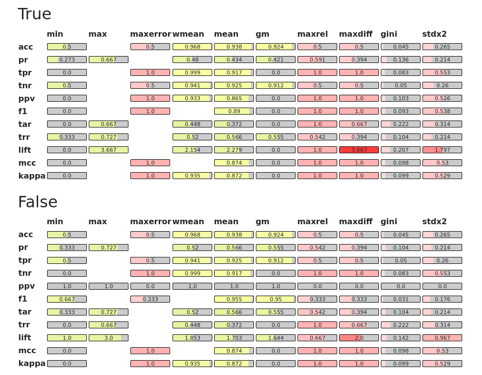
This is similar to the HtmlTable environment, with the difference that Plotly is used for heatmap plotting of the values.
ToJson
When provided as an environment to the show method, it does
not create any visual output but instead returns a string
that is a json damp of the report values. This can be used
to reconstruct the report like so:
import fairbench as fb
import json

# serialize a report
json_dump = report.show(env=fb.export.ToJson)
# deserialize
dicts_and_lists = json.loads(json_dump)
reconstructed = fb.core.Value.from_dict(dicts_and_lists)