Full reports
Before starting, install FairBench with the following command. This can assess any system. Install extras are available to optionally run computer vision, graph, and LLMs benchmarks.
pip install fairbench
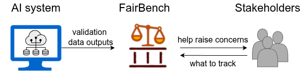
This tutorial shows how to bootstrap fairness analysis for a new AI system using FairBench. In particular, the recommended workflow is to first identify prospective fairness concerns, and then decide which of those matter (human-in-the-loop, consult with stakeholders). Afterwards, keep track of important concerns with standalone measures covered in the overview.
Most steps described in this tutorial can be explored via a browser interface. This can be started via the following command, and even customized to include experiment setups of your own. The interface can also export FairBench code for running the same pipeline programmatically, without needing to wade through the documentation.
python -m fairbench.bench.wizard
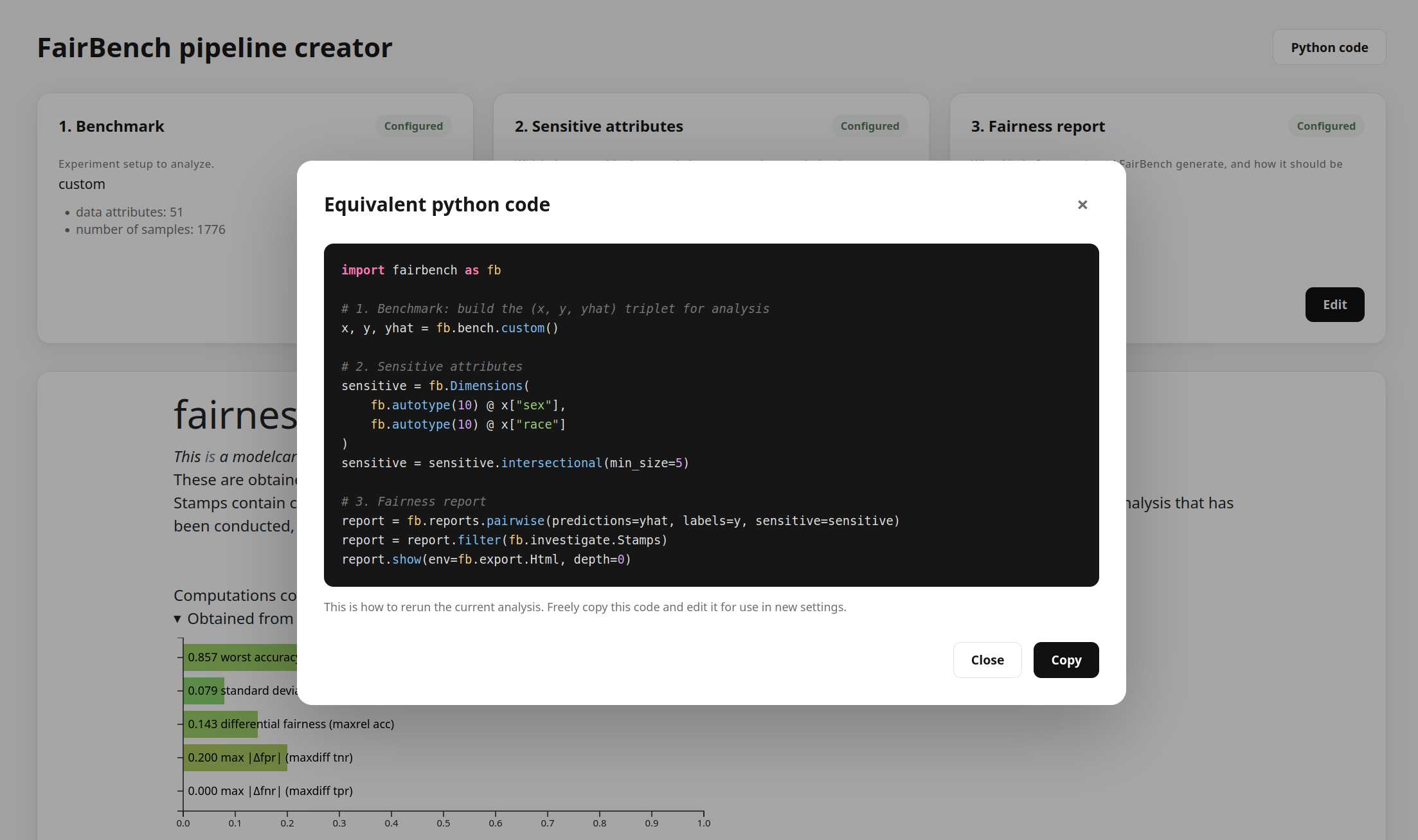
How ro run the pipeline creator with custom setups.
Given a function that runs your experiment setup, manually start a wizard that contains custom experiment setups like below. Setups declared this way are processed through the whole pipeline. Of the outputs, `y` and `yhat` should duck-type iterables and `x` a dictionary of categorical or numerical columns.import fairbench as fb
from fairbench.bench.wizard import BENCH_REGISTRY
BENCH_REGISTRY["custom"] = {
"label": "Custom experiment (declared programmatically)",
"func": lambda: fb.bench.tabular.compas(),
}
if __name__ == "__main__":
fb.bench.serve_wizard(port=8000)
1. Prepare data
To assess your system, start by generating predictions for test data. Here we evaluate a binary classifier that is available for out-of-the-box experimentation; outputs are the test portion of the dataset x, the target binary labels y, and binary predicted labels yhat. We are interested in seeing how fair those predictions are.
import fairbench as fb
test, y, yhat = fb.bench.tabular.adult()
2. Sensitive attributes
Pack sensitive attributes found across test samples into a data structure holding multiple dimensions. This stores any number of attributes with any number of values by considering each value as a separate dimension.
In particular, each dimension is a binary or fuzzy array whose i-th element represents whether the i sample has the attribute corresponding to the dimension. One construction pattern is the following. This first analyses categorical iterables and then packs them into dimensions. It then computes all non-empty intersections that combine attributes, and finally retains the most specialized intersectional subgroups.
sensitive = fb.Dimensions(fb.categories @ test[8], fb.categories @ test[9])  # analyse the gender and race columns
sensitive = sensitive.intersectional()  # automatically find non-empty intersections
sensitive = sensitive.strict()  # no fully ovrelapping intersections (e.g., remove Male if there is Male&Other)
print(sensitive)
Male&Native American           [0 0 0 ... 0 0 0]
Male&Other                     [0 1 0 ... 0 0 0]
Male&Caucasian                 [0 0 0 ... 1 0 0]
Male&African-American          [1 0 0 ... 0 0 0]
Male&Hispanic                  [0 0 1 ... 0 0 0]
Female&Native American         [0 0 0 ... 0 0 0]
Female&Other                   [0 0 0 ... 0 0 0]
Female&Caucasian               [0 0 0 ... 0 0 1]
Female&African-American        [0 0 0 ... 0 1 0]
Female&Hispanic                [0 0 0 ... 0 0 0]
One can apply numpy functions on each column, for example to
retrieve the number of samples in each dimension. There is
already a problematic intersection of only one data sample,
for which results degrade to statistical noise.
Small groups should be skipped
by instead retrieving intersections(min_size=10),
but we do not do so here for the sake of brevity.
Pay attention how this neglect affects subsequent
assessments.
print(sensitive.sum())
Female&Native American         1
Female&Other                   38
Female&African-American        335
Female&Caucasian               270
Female&Hispanic                51
Male&Native American           5
Male&Other                     159
Male&African-American          1458
Male&Caucasian                 971
Male&Hispanic                  249
3. Compute reports
Use sensitive attributes alongside predictions to generate fairness reports. Below is one that compares all pairs of population groups or subgroups according to a wide range of base performance measures. Reports can be viewed under various visualization environments.
The comparisons for each measure (row) are reduced to one value with reduction strategies (columns). For example, the value at column min and row acc indicates the minimum accuracy across all sensitive groups. Similarly, the value at column maximum relative difference maxrel and row positive rate pr indicate the maximum relative difference between the positive rates of all groups; this is the differential fairness extension to the well-known prule measure originally coined for binary sensitive attributes (see below).
report = fb.reports.pairwise(predictions=yhat, labels=y, sensitive=sensitive)
report.show(env=fb.export.ConsoleTable)
                                           min          max     maxerror        wmean         mean           gm        pnorm       maxrel      maxdiff         gini        stdx2
acc                                      0.959                     0.041        0.968        0.978        0.978            3        0.041        0.041        0.008        0.027
pr                                       0.241        0.667                     0.475        0.442        0.424            1        0.638        0.425        0.157        0.250
tpr                                          1            1            0            1            1            1            3            0            0            0            0
tnr                                      0.912                     0.088        0.939        0.964        0.964            3        0.088        0.088        0.014        0.050
ppv                                      0.857                     0.143        0.932        0.942        0.942            2        0.143        0.143        0.022        0.078
f1                                       0.923                     0.077                     0.970        0.970            3        0.077        0.077        0.011        0.042
gmi                                      0.926                     0.074                     0.971        0.970            3        0.074        0.074        0.011        0.040
tar                                      0.207        0.667                     0.443        0.420        0.399            1        0.690        0.460        0.172        0.264
trr                                      0.333        0.759                     0.525        0.558        0.543            1        0.561        0.425        0.124        0.250
lift                                         1            4                         2            2            2            8        0.638            2        0.159            1
mcc                                      0.905                     0.095                     0.953        0.953            3        0.095        0.095        0.017        0.059
kappa                                    0.901                     0.099        0.933        0.952        0.951            3        0.099        0.099        0.018        0.061
Info
The task type and applicable measures are determined by the report's arguments. There exist other report types too! Read more in the report documentation.
See the comprehensive list of all
measures and reductions,
but you can find out what the abbreviations refer
to by either using a visualization environment
that prints such information (see next section)
or simply calling report.help() to view lengthier
descriptions of all factors contributing to
the generated report.
report.help()
##### FairBench help #####
Access the following fields of the selected value to explore results:
- value.min                 This reduction is the minimum.
- value.acc                 This measure is the accuracy.
- value['Female&African-American'] This is the value for group 'Female&African-American'.
- value.samples             This is the sample count.
- value.ap                  This count is the actual positive labels.
- value.an                  This count is the actual negative labels.
- value.tp                  This count is the true positive predictions.
- value.tn                  This count is the true negative predictions.
- value['Female&Hispanic']  This is the value for group 'Female&Hispanic'.
- value['Female&Other']     This is the value for group 'Female&Other'.
- value['Female&Caucasian'] This is the value for group 'Female&Caucasian'.
- value['Female&Native American'] This is the value for group 'Female&Native American'.
- value['Male&African-American'] This is the value for group 'Male&African-American'.
- value['Male&Hispanic']    This is the value for group 'Male&Hispanic'.
- value['Male&Other']       This is the value for group 'Male&Other'.
- value['Male&Caucasian']   This is the value for group 'Male&Caucasian'.
- value['Male&Native American'] This is the value for group 'Male&Native American'.
- value.pr                  This measure is the positive rate.
- value.positives           This count is the positive predictions.
- value.tpr                 This measure is the true positive rate/recall/sensitivity/hit rate.
- value.tnr                 This measure is the true negative rate/specificity.
- value.negatives           This count is the negative predictions.
- value.ppv                 This measure is the positive predictive value/precision.
- value.f1                  This measure is the f1 score.
- value.gmi                 This measure is the geometric mean of tpr and tnr - accounts for class
|imbalance.
- value.tar                 This measure is the true acceptance ratio (true positives compared to all).
- value.trr                 This measure is the true rejection ratio (true negatives compared to all).
- value.lift                This measure is the lift ratio (tpr divided by pr).
- value.mcc                 This measure is the Matthews correlation coefficient.
- value.kappa               This measure is the Cohen's Kappa score.
- value.max                 This reduction is the maximum.
- value.maxerror            This reduction is the maximum deviation from the ideal value.
- value.wmean               This reduction is the weighted average.
- value.mean                This reduction is the average.
- value.gm                  This reduction is the geometric mean.
- value.pnorm               This reduction is the p-norm (default L2).
- value.maxrel              This reduction is the maximum relative difference.
- value.maxdiff             This reduction is the maximum difference.
- value.gini                This reduction is the gini coefficient.
- value.stdx2               This reduction is the standard deviation x2.
4. Go into details
Almost every computation, including standalone measures, is a FairBench report that keeps track of internal values. Thus, starting from a top-level view, one can delve deeper into report details by specializing and -as covered in the next section- filtering results. The outcome is sub-reports. The final report is visualized in various comprehensive formats, in either the console or in the browser.
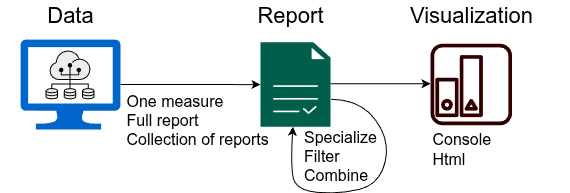
Explore reports by focusing on any of their contributing
computations. Use the programmatic dot notation to do this.
report.help() shows what you can specialize on. You can
even chain multiple specializations! Fallback to
dictionary access notation if the dot notation would be invalid
(e.g., when the specialization includes spaces or special
characters).
Example: report.acc.min is equivalent to
report["acc"]["min"] and retrieves a first sub-report
for the accuracy, and then a sub-sub-report for the minimum
accuracy. Tha latter happens to be a measure value.
This is not the end, however, and the sub-sub-report
can be specialized further like below.
You can also skip levels of the hierarchy, for example
by writing report.tp to retrieve the true positive values that
have contributed to all computations (there could be many
repetitions of those).
Next is an example with console output, though there are more visualization environments. In the example, we focus on the minimum accuracy to keep the outcome simple. All visualization environments work with reports, or even collections of reports, which are also reports.
report.min.acc.show(env=fb.export.Console)
This is the console output:
##### acc #####
|This measure is the minimum of the accuracy.
|Value: 0.929 min acc

  (0.0, 1.0)
  ▎    █  █  █           █
  ▎ ▆  █  █  █  ▆  ▆  ▆  █  ▆  ▄  ▆  ▆
  ▎ █  █  █  █  █  █  █  █  █  █  █  █
  ▎ █  █  █  █  █  █  █  █  █  █  █  █
  ▎ █  █  █  █  █  █  █  █  █  █  █  █
  ▎▬*▬▬-▬▬+▬▬x▬▬o▬▬□▬▬◇▬▬#▬▬@▬▬%▬▬&▬▬|
                           (12.0, 0.0)

   * Female&Caucasian                    0.978 acc
   - Female&Native American              1 acc
   + Female&Other                        1 acc
   x Female&Asian                        1 acc
   o Female&African-American             0.985 acc
   □ Female&Hispanic                     0.959 acc
   ◇ Male&Caucasian                      0.971 acc
   # Male&Native American                1 acc
   @ Male&Other                          0.973 acc
   % Male&Asian                          0.929 acc
   & Male&African-American               0.961 acc
   | Male&Hispanic                       0.981 acc
5. Simplify reports
FairBench provides filters that enhance report outcomes. For example, they can remove entries that do not violate a given threshold, leaving only problematic values behind.
A particularly noteworthy filter, which is presented below, are fairness stamps. These refer to a few types of fairness evaluation that are prevalent in the literature. However, they are accompanied by caveats and recommendations that turns them into a fairness modelcard.
Filtering through reports yields new ones that can be manipulated
and viewed normally. Below, the Html environment is used
to save and/or open a report in the browser
the generated HTML representation of reports. The generated document
requires an internet connection to properly view, as it depends
on bootstrap for theming. Html-based environments are
counterparts to console options.
report = report.filter(fb.investigate.Stamps)
report.show(env=fb.export.Html(horizontal=True), depth=1)
Info
The provided depth parameter controls the level of detail. Default depth
is zero, which automatically selects the shallowest meaningful
level of detail.
The following page opens in the browser, and you can explore it here too:
Danger
Blindly following filters may neglect certain kinds of evaluation. Icons also give an indication of which are the most problematic values, but any measure value could be worrisome. Therefore, computed values are also shown.